This notebook compares the performance of the new capped distance functions in MDAnalysis.lib.distances against the existing functions.

These functions were implemented as part of Google Summer of Code 2018 by Ayush Suhane a graduate student at the University of British Columbia, Canada, with help from Richard J Gowers, Jonathan Barnoud and Sébastien Buchoux.

We will look at two cases, which are similar to finding bonds and radial distribution functions.

This notebook was prepared using a development version of 0.19.3 of MDAnalysis. The capped distance functions are available in version 0.19.0 onwards.

import numpy as np
import MDAnalysis as mda
from MDAnalysis.lib.distances import (
    capped_distance, distance_array,
    self_capped_distance, self_distance_array
)

import matplotlib.pyplot as plt
%matplotlib notebook

import seaborn as sns
sns.set_context('notebook')

print(mda.__version__)

0.19.3-dev

We will first define a function to generate random coordinates for a given box size. These coordinates will have a typical particle density for atomistic soft matter molecular simulations.

# typical atomistic particle density
# 4055 water atoms in 5nm cube
density = 4055 / (50. ** 3)

def make_coords(boxsize): # boxlength in A
    # makes 3d coordinates in cube of boxsize side length
    n = int((boxsize ** 3) * density)
    crds = np.random.random(n * 3).reshape(n, 3) * boxsize
    
    return crds.astype(np.float32)

guessing bonds

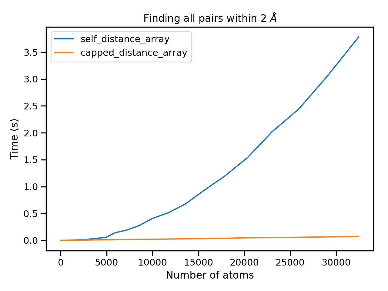
To guess which atoms are bonded (usually due to missing information in the topology) we have to find all pairwise distances within 2A. (These distances are then further processed to match a particular distance for a given pairing of atom types)

Here we generate different box sizes from 20 to 75 A, timing how long to find all pairwise distances within 2A. We are using the self_ variant of the distance methods as we are comparing an array of coordinates only with itself.

natoms = []
brute = []
capped = []
capped_nod = []

for boxsize in np.linspace(10, 100, 26):
    a = make_coords(boxsize)
    
    natoms.append(a.shape[0])
    
    t = %timeit -o -q self_capped_distance(a, max_cutoff=2)
    capped.append(t)
    
    t = %timeit -o -q self_distance_array(a)
    brute.append(t)

We see that the capped variant is substantially faster, whilst the brute force method is scaling $\mathcal{O}(n^2)$ as expected.

fig, ax = plt.subplots()

ax.plot(natoms, [t.average for t in brute], label='self_distance_array')
ax.plot(natoms, [t.average for t in capped], label='capped_distance_array')

ax.legend()

ax.set_title('Finding all pairs within 2 $\AA$')
ax.set_xlabel('Number of atoms')
ax.set_ylabel('Time (s)')

fig.tight_layout()

RDF test

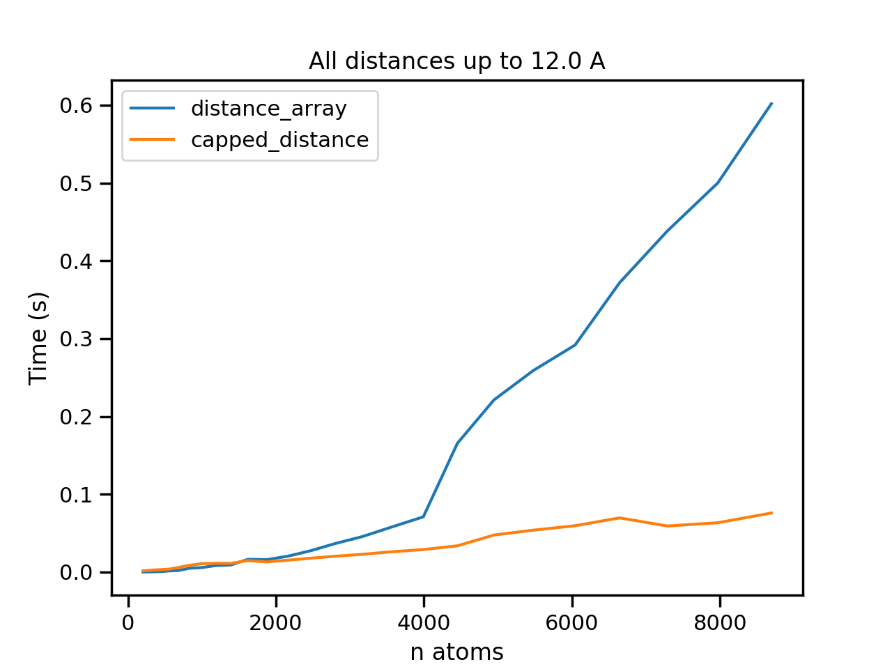
Here we test finding all pairwise distances up to 12.0 A between two sets of coordinates. This is a proxy for a radial distribution function, where we want to know the probability distribution of pairwise distances between two chemical species.

The particle density is now reduced by a factor of 20, and boxsizes vary from 50 to 175 A cubes.

rdf_cutoff = 12.0

natoms_rdf = []
brute_rdf = []
capped_rdf = []

for boxsize in np.linspace(50, 175, 26):
    c = make_coords(boxsize)
    s1, s2 = c[::20], c[5::20]
    
    t_brute = %timeit -o -q distance_array(s1, s2)
    t_capped = %timeit -o -q capped_distance(s1, s2, max_cutoff=rdf_cutoff)
    
    brute_rdf.append(t_brute)
    capped_rdf.append(t_capped)
    
    natoms_rdf.append(s1.shape[0])

fig, ax = plt.subplots()

ax.errorbar(natoms_rdf, [t.average for t in brute_rdf], label='distance_array')
ax.errorbar(natoms_rdf, [t.average for t in capped_rdf], label='capped_distance')

ax.set_title('All distances up to 12.0 A')
ax.set_ylabel('Time (s)')
ax.set_xlabel('n atoms')

ax.legend()

Conclusion

The new capped functions in lib.distances are much faster! They also impement quite complicated algorithms with minimal difficulty to a user; all that is required is to define a maximum “interesting” distance, which is often known. Ie for bonds we weren’t interested in distances larger than 2A, for an RDF often 12A is enough.

These benchmarks represent only the first iteration of this functions, and it is anticipated that further optimisations can be made to these.